Part 3: The Pair Selection Puzzle

Asking the right questions when you can't ask them all

---

Where We Left Off

Part 1 set up the problem: 237 pendants, pairwise comparisons. Part 2 covered TrueSkill—how $\mu$ tracks estimated appeal and $\sigma$ tracks uncertainty.

Now the real question: which pairs should we actually compare?

---

The Explore-Exploit Problem

Twenty comparisons in, the app knows a few things:

• Pendant #47 (rose gold teardrop) has won 6 of 7 matches. Looking good.
• Pendant #183 has never been compared. Complete mystery.
• Pendant #12 has mixed results across 5 comparisons. Meh confidence.

What should we show next?

Option A: Exploit
Compare #47 against its closest rivals. Nail down the top of the ranking.

Option B: Explore
Compare #183 (never seen) against something. Maybe it's a hidden gem?

Classic exploration-exploitation tradeoff.^[1]

Figure 1: The fundamental tradeoff. Pure exploitation might miss better options; pure exploration wastes comparisons on known mediocre items.

Too much exploitation → miss better options hiding in the unexplored pile.

Too much exploration → waste comparisons on stuff you already know is mediocre.

We need a principled way to balance.

---

The Obvious Ideas (And Why They Fail)

Random pairs: Just pick any two.

• ❌ Wastes comparisons on items we already understand
• ❌ Shows obviously mismatched pairs (uninformative)
• ❌ Repeats the same pair too often

Round-robin: Always compare items with the fewest comparisons.

• ✅ Every item gets exposure
• ❌ Doesn't care about match quality (#1 vs #200 teaches nothing)
• ❌ Ignores uncertainty—some items need more matches than others

Similar-$\mu$ heuristic: Compare items with close mean values.

• ✅ Close matches are informative
• ❌ Ignores uncertainty ($\sigma$)
• ❌ Gets stuck on the same competitive pairs
• ❌ Never explores new items

We need something smarter.

---

$E[\Delta\sigma]$: Expected Uncertainty Reduction

Here's the insight from Bayesian active learning: pick the pair that teaches us the most.

But "teaches us the most" is vague. How do we measure it?

Answer: measure how much uncertainty will shrink.

For any pair (i, j), compute the expected $\Delta\sigma$—the expected reduction in total uncertainty after comparing them.

$$E[\Delta\sigma]_{i,j} = \sum_{y \in \{L, R, D\}} P(y) \cdot \Delta\sigma_y$$

Where:

• $y$ is the outcome: Left wins (L), Right wins (R), Draw (D)
• $P(y)$ is the probability of that outcome
• $\Delta\sigma_y$ is how much uncertainty drops if that outcome happens

How to Compute It

TrueSkill gives us the tools. For pendants with ratings $(\mu_L, \sigma_L)$ and $(\mu_R, \sigma_R)$:

1. Get outcome probabilities: TrueSkill predicts $P(\text{Left wins})$, $P(\text{Right wins})$, $P(\text{Draw})$ based on the $\mu$ gap and combined uncertainty.

2. Simulate each outcome: Run the TrueSkill update for each possible result to see what $\sigma$ values would become.

3. Take the expectation:

   $$E[\Delta\sigma] = \sum_{y} P(y) \cdot (\sigma_\text{before} - \sigma_\text{after}(y))$$

Why It Works

This formula captures what we want:

Situation	$E[\Delta\sigma]$	Why
Both items uncertain	High	Lots of uncertainty to reduce
One item uncertain	Medium	Still something to learn
Both items well-known	Low	Not much uncertainty left
Close match (similar $\mu$)	Higher	Uncertain outcome = balanced learning
Lopsided match	Lower	Predictable outcome = less info

No heuristics or special cases. The math just does the right thing.

---

Thompson Sampling: Randomness on Purpose

$E[\Delta\sigma]$ is great, but it's deterministic. Same state → same pair every time.

That causes problems:

• Gets stuck in loops
• Over-focuses on a small set of "most informative" pairs
• Misses items that would be informative with a bit more exploration

Enter Thompson Sampling, an algorithm from 1933 (!) that's still one of the best explore-exploit balancers we have.

How It Works

1. For each pendant, sample an appeal value from its posterior: $\text{sample} \sim \mathcal{N}(\mu, \sigma^2)$
2. Sort pendants by sampled appeal
3. Look at adjacent pairs in this sampled ranking
4. Score those pairs by $E[\Delta\sigma]$, pick the best

Why It's Clever

The sampling is the key:

• High-$\sigma$ items → wide distributions → samples bounce around wildly

• Sometimes they sample high (top of ranking), sometimes low (bottom)

• They naturally end up in more comparisons

• Low-$\sigma$ items → narrow distributions → samples stay consistent

• They hold their position

• Only get compared when they're actually competitive

Figure 2: High-uncertainty items have wide posterior distributions, causing their samples to fluctuate. This naturally leads to more exploration of uncertain items.

Thompson Sampling is a natural explore-exploit balance: uncertain items get explored, certain items only compete when relevant.

---

The Hybrid: Best of Both

Pure $E[\Delta\sigma]$ is too greedy. Pure Thompson is too random.

So we combine them:

if random() < 0.25:
    candidates = thompson_sample_pairs()  # Sample from posteriors
else:
    candidates = all_pairs()              # All O(n²) pairs

best = max(candidates, key=expected_sigma_reduction)
return best

• 75% of the time: Greedy $E[\Delta\sigma]$ on all pairs
• 25% of the time: Thompson generates candidates, then $E[\Delta\sigma]$ picks the best

This gives us efficiency from the greedy approach, exploration from Thompson, and no loops.

Figure 3: The hybrid selection algorithm. 75% of comparisons use greedy $E[\Delta\sigma]$ optimization; 25% use Thompson Sampling to avoid local optima.

---

Cooldowns for Skips and Draws

One more thing: if you skip a pair or call it a draw, we exclude that pair from the next 2 rounds. Prevents annoying repeats while still letting informative pairs resurface later.

---

The Complete Flow

Putting it together:

Figure 4: The complete pair selection algorithm, from initialization through scoring and filtering.

---

Does It Actually Work?

I tested the hybrid approach on my 237 pendants.

Before (random pairs):

• 100+ comparisons before rankings stabilized
• Kept showing obviously mismatched pairs
• Top 3 kept changing after 80 comparisons

After (hybrid $E[\Delta\sigma]$ + Thompson):

• ~50 comparisons to stable top 10
• Pairs felt meaningful—close calls that were hard to decide
• Top 3 locked in by comparison #45

Every pair feels like it matters. No more wasted clicks.

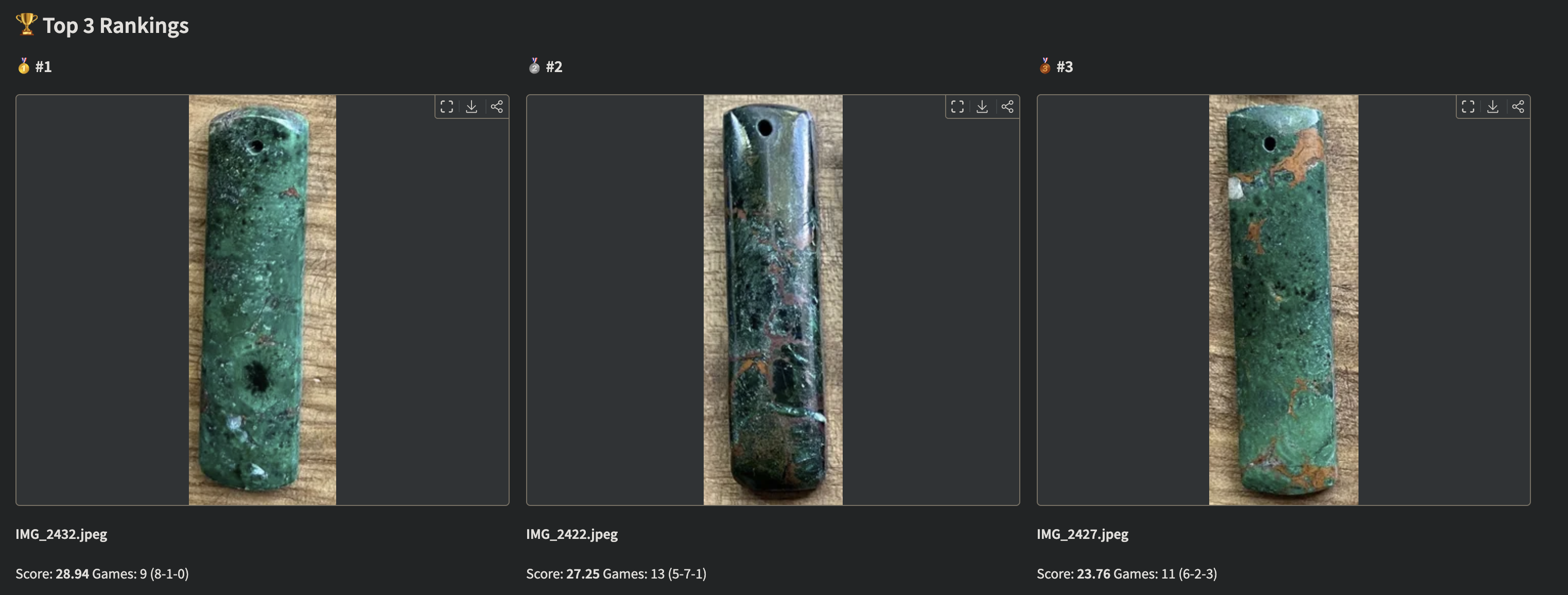
Figure 5: The final leaderboard, ranked by conservative score ($\mu - 3\sigma$). The top 3 are clearly separated with high confidence after just 47 comparisons.

---

Summary

1. $E[\Delta\sigma]$ is the gold standard for active learning in pairwise ranking. It directly measures expected information gain.

2. Thompson Sampling adds healthy randomness by sampling from posteriors, naturally balancing exploration and exploitation.

3. The hybrid (75% $E[\Delta\sigma]$, 25% Thompson) combines their strengths.

4. TrueSkill does the heavy lifting. quality_1vs1() and rate_1vs1() handle all the probabilistic reasoning.

5. Cooldowns prevent annoyance. Nobody wants to see the same pair twice after skipping.

---

Epilogue

After 47 comparisons, the app converged. My top 3:

1. 🥇 Rose gold teardrop with subtle diamond accent
2. 🥈 Minimalist gold circle (surprisingly close)
3. 🥉 Vintage-inspired cameo with modern twist

Went with #1. Valentine's Day was saved.

And somewhere in there, I learned more about Bayesian statistics than any textbook taught me. Sometimes the best way to learn is to have a problem you actually care about.

---

References

---

Source code: github.com/hugocool/product_picker

Previous: Part 2 - TrueSkill Demystified

Start from the beginning: Part 1 - The Pendant Problem

---

1. Sutton, R. S., & Barto, A. G. (2018). Reinforcement Learning: An Introduction (2nd ed.). MIT Press. The explore-exploit tradeoff is foundational in bandit problems and sequential decision making. ↩︎